The staggered finite-difference method (交错网格有限差分方法)

2022年2月28日2022年2月28日 numanal 2 个评论交错网格, 有限差分

One-dimensional problem

We consider 1d model problem for acoustic problem:\[ \frac{\partial u}{\partial t} – \frac{\partial v}{\partial x} =0, \quad \frac{\partial v}{\partial t} – \frac{\partial u}{\partial x} =0. \tag{1}\]

FD scheme

Let \(u_i^n \) be the approximation of \(u(x_i, t_n)\) for the uniform mesh with \(x_i=i h, t^n = n \tau\). The finite difference scheme can be expressed as follows\[\begin{align} \frac{u_i^{n+\frac{1}{2}}-u_i^{n-\frac{1}{2}}}{\tau} – \frac{v_{i+\frac{1}{2}}^n – v_{i-\frac{1}{2}}^n}{h} =0 , \\ \frac{v_{i+\frac{1}{2}}^{n+1}-v_{i+\frac{1}{2}}^{n}}{\tau} – \frac{u_{i+1}^{n+\frac{1}{2}} – u_{i}^{n+\frac{1}{2}}}{h} =0 . \end{align} \tag{2}\] For other schemes, see, e.g., [1].

We can interpret (2) in another viewpoint. Making a integration of \(u_t-v_x=0\) on the interval \((x_{i-1/2}, x_{i+1/2})\), we have\[ \int_{x_{i-1/2}}^{x_{i+1/2}} \frac{\partial u}{\partial t}(x,t_n) dx = \int_{x_{i-1/2}}^{x_{i+1/2}} \frac{\partial v}{\partial x}(x,t_n) dx =v(x_{i+1/2},t_n)-v(x_{i-1/2},t_n).\]By using the mid-point quadrature formula, we have (note \(x_{i+1/2}-x_{i-1/2}=h\))\[ h \frac{\partial u}{\partial t}(x_i,t_n) = v(x_{i+1/2},t_n)-v(x_{i-1/2},t_n).\]Next, using the center difference formula for \(\frac{\partial u}{\partial t} \) at \(t_n\) leads to (note \(t_{n+1/2}-t_{n-1/2}=\tau\))\[ h \frac{u(x_i,t_{n+1/2})-u(x_i,t_{n-1/2})}{\tau} = v(x_{i+1/2})-v(x_{i-1/2}), \tag{3}\]which is the same as (2).

Numerical results

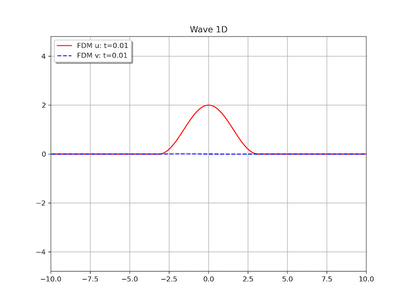
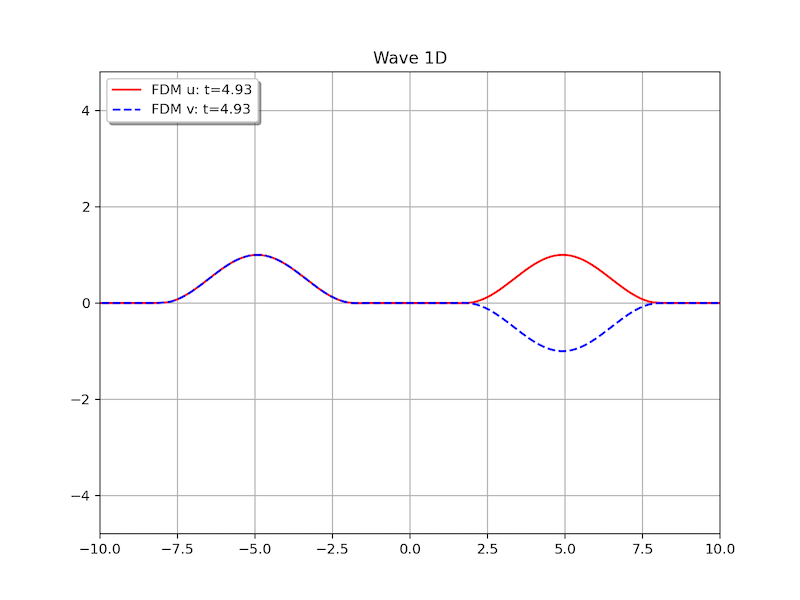
Example 1 (Homogenous BC, [1]). Let \(\Omega=[-L,L]\). Suppose the acoustics has the pressure\[ u(x,0)=\begin{cases} 1-\cos (x+\pi), & \text{if } |x|\leq \pi, \\ 0, & \text{if } \pi <|x|\leq L, \\ \end{cases}\]The boundary condition is set to be zero, i.e., \(u(-L,t)=u(L,t)=0\). The velocity satisfies \(v(x,0)=0\) for all \(x\in \Omega\). In numerical test, we set \(L=10\).

Example 2 (Non-homogenous BC). Let \(\Omega=(0,b)\). Suppose the acoustics has the boundary condition:\[ \begin{cases} u(0,t)=\sin t, \\ u(b,t)=0, \end{cases}\quad \begin{cases} v(0,t)=0, \\ v(b,t)=0. \end{cases} .\]The initial conditions are set to be zero, i.e., \(u(x,0)=v(x,0)=0\). The velocity satisfies \(v(x,0)=0\) for all \(x\in \Omega\).

Two-dimensional problem

Given a bounded rectangular domain \(\Omega\subset \mathbb{R}^2\). We consider 2d model problem for acoustic problem: Find \(u\in \mathbb{R},\mathbf{v}=[v,w]^T\in \mathbb{R}^2\) s.t.\[ \frac{\partial u}{\partial t} – \nabla\cdot \mathbf{v} =0, \quad \frac{\partial \mathbf{v}}{\partial t} – \nabla u = 0,\quad \text{in }\Omega.\]

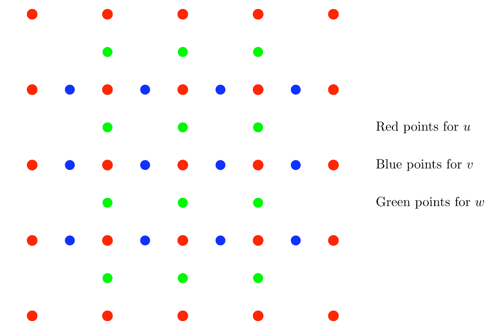
Staggered FD scheme 2D

Let \(u_{i,j}^n\) be the approximation of \(u(x_i, y_i, t_n)\) for the uniform mesh with \(x_i=i h, y_j=jh, t^n = n \tau\). The staggered finite difference scheme can be expressed as follows\[ \frac{u_{i,j}^{n+\frac{1}{2}}-u_{i,j}^{n-\frac{1}{2}}}{\tau} – \frac{v_{i+\frac{1}{2},j}^n – v_{i-\frac{1}{2},j}^n}{h} – \frac{w_{i,j+\frac{1}{2}}^n – w_{i,j-\frac{1}{2}}^n}{h} = 0, \\ \frac{v_{i+\frac{1}{2},j}^{n+1}-v_{i+\frac{1}{2},j}^{n}}{\tau} – \frac{u_{i+1,j}^{n+\frac{1}{2}} – u_{i,j}^{n+\frac{1}{2}}}{h} =0,\\ \frac{w_{i,j+\frac{1}{2}}^{n+1}-w_{i,j+\frac{1}{2}}^{n}}{\tau} – \frac{u_{i,,j+1}^{n+\frac{1}{2}} – u_{i,j}^{n+\frac{1}{2}}}{h} =0.\]For the first step \(n=0\), we change the update procedure for \(u\) to be\[ \frac{u_{i,j}^{n+\frac{1}{2}}-u_{i,j}^{n}}{\tau/2} – \frac{v_{i+\frac{1}{2},j}^n – v_{i-\frac{1}{2},j}^n}{h} – \frac{w_{i,j+\frac{1}{2}}^n – w_{i,j-\frac{1}{2}}^n}{h} = 0.\]

After allocating memory for \(u_{(N_x+1)\times (N_y+1)}, v_{N_x\times (N_y-1)}, v_{(N_x-1)\times N_y} \) and updating \(u^{1/2}\), the main step is to follow the FD scheme. The kernel code is as the following (don’t forget to impose boundary condition after each updating):

for i in range(0,Nx):
    for j in range(1,Ny):
        v[i,j-1] += (u[i+1,j]-u[i,j])*dt/dx

for i in range(1,Nx):
    for j in range(0,Ny):
        w[i-1,j] += (u[i,j+1]-u[i,j])*dt/dx

for i in range(1,Nx):
    for j in range(1,Ny):
        u[i,j] += (v[i,j-1]-v[i-1,j-1])*dt/dx + (w[i-1,j]-w[i-1,j-1])*dt/dy

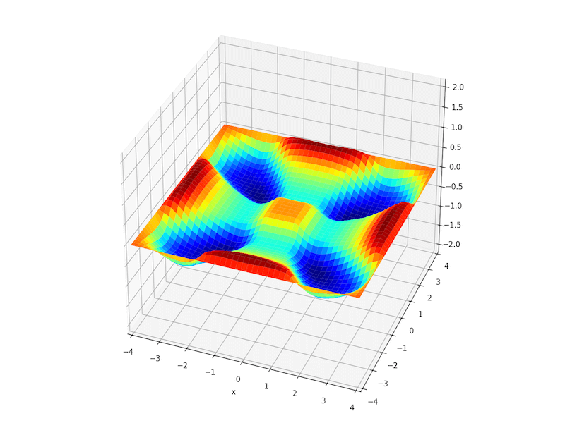
Example 3 (homogenous BC). Let \(\Omega=[-4,4]\times[-4,4]\). Suppose the acoustics has the initial pressure\[ u(x,y,0)=\begin{cases} 1+\cos (x^2+y^2), & \text{if } x^2+y^2\leq \pi, \\ 0, & \text{if } \pi < x^2+y^2 \leq 4. \end{cases}\]The boundary condition is set to be zero, i.e., \(u(x,y,t)=0,\ x\in \partial \Omega\). The initial velocity satisfies \(v(x,0)=0\) for all \(x\in \Omega\).

References

[1] Maria Yuliani Danggo and Sudi Mungkasi. A staggered grid finite difference method for solving the elastic wave equations. 2017. J. Phys.: Conf. Ser. 909 012047.

Appendix: Python code for Example 1 and 2.

# Staggered finite difference method for acoustic wave.
# u_t - v_x = 0,   v_t - u_x = 0, in [-L,L]
# u(-L,t) = u(L,t) = 0.
# 
# class list:
#   Wave1d - pde class
#   Mesh - for mesh
#   Wave1DSolver - Solver
# 
# -- https://numanal.com 2022/2/2
# 
import numpy as np
import matplotlib.pyplot as plt


class Wave1d(object):
    # pde class
    def __init__(self, a, b, T):
        self.a = a
        self.b = b
        self.umax = 4
        self.T = T

    def u(self,x,t):
        pass

    def u_l(self,t):
        # return 0.*t # ex1
        return np.sin(np.pi*.5*t) # ex2
    def u_r(self,t):
        return 0.*t

    def u0(self,x):
        # ex1
        # r = 0*x
        # for i in range(r.shape[0]):
        #     if np.abs(x[i]) <= np.pi:
        #         r[i] = 1-np.cos(x[i]+np.pi)
        # return r
        # ex2
        return 0*x
    
    def v0(self,x):
        return 0.*x
    
    def f(self,x,t):
        return 0.*x


# uniform spatial and time space
class Mesh():
    def __init__(self,x,t):
        self.x = x
        self.t = t


# solver class
class Wave1DSolver():
    def __init__(self, pde, mesh):
        self.pde = pde
        self.mesh = mesh
        self.Nx = mesh.x.shape[0]-1
        self.Nt = mesh.t.shape[0]-1
        self.dx = mesh.x[1]-mesh.x[0]
        self.dt = mesh.t[1]-mesh.t[0]
        
    def solve(self):
        dt, dx = self.dt, self.dx
        Nx = self.Nx

        # set initial values
        x = self.mesh.x
        u = self.pde.u0(x)             # current u
        v = self.pde.v0(x[:-1]+dx*.5)  # current v (staggered mesh)
        
        # compute u^{1/2}
        for i in range(1,Nx):
            u[i] = u[i] + (v[i]-v[i-1])*.5*dt/dx
        # impose boundary condition
        u[0] = self.pde.u_l(dt*.5)
        u[-1] = self.pde.u_r(dt*.5)

        # gif plot - 1/3
        plt.figure(figsize=(8, 6), dpi=80)
        plt.ion()
        
        for j in range(1,self.Nt):
            for i in range(0,Nx):
                v[i] += (u[i+1]-u[i])*dt/dx
            for i in range(1,Nx):
                u[i] += (v[i]-v[i-1])*dt/dx
            
            # u(a,t) and u(b,T)
            u[0] = self.pde.u_l(dt*(j+.5))
            u[-1] = self.pde.u_r(dt*(j+.5))
            
            # gif plot - 2/3
            if j%np.ceil(t.shape[0]/50) == 1:
                plt.cla()
                plt.title("Wave 1D")
                plt.grid(True)
                plt.plot(x,u, '-r', label="FDM u: t="+str(int(1e5*self.mesh.t[j+1])/1e5))
                plt.plot(x[:-1]+.5*dx,v, '--b', label="FDM v: t="+str(int(1e5*self.mesh.t[j+1])/1e5))
                plt.xlim(x[0], x[-1])
                plt.ylim(-1.2*self.pde.umax, 1.2*self.pde.umax)
                plt.legend(loc="upper left", shadow=True)
                plt.pause(.1)
            
        # gif plot - 3/3
        plt.ioff()
        plt.show()

        return 0


if __name__ == "__main__":
    pde = Wave1d(a=0, b=6, T=10.)  # pde
    Nx = 200        # Nx
    x = np.linspace(pde.a, pde.b, num=Nx, endpoint=True)
    dt = 0.05*(pde.b-pde.a)/Nx; print(dt)
    Nt = int(pde.T/dt+1); print(Nt)
    t = np.linspace(0, pde.T, num=Nt, endpoint=True)
    mesh = Mesh(x, t)

    solver = Wave1DSolver(pde, mesh)
    solver.solve()

分享到: