帕德逼近 (Padé approximation)

引言

Padé 逼近多项式 \(R_{n,m}(x)=\frac{P_n(x)}{Q_m(x)}\) 具有形式\[ R_{n,m}(x) = \frac{p_0+p_1x+\cdots+p_nx^n}{1+q_1x+\cdots+q_mx^m} =\frac{\sum_{j=0}^n p_jx^j }{1+\sum_{k=1}^m q_kx^k}. \tag{1}\]它可从如下给定幂级数 (或仅仅是形式定义) 得到\[ f(x):=\sum_{k=1}^{\infty}c_kx^k.\]基本原理为, 给定两个整数 \(m,n\in \mathbb{N}\cup \left\{ 0 \right\}\) 可以找到阶数小于或等于 \(n\) 和 \(m\) 的多项式 \(P_n(x)\) 和 \(Q_m(x)\), 使得两个级数 \(Q_m(x)f(x)-P_n(x)\) 与 \(f(x)\) 尽可能多的重合. 事实上, 就是要求 [1]\[ Q_m(x) f(x)-P_n(x) = O(x^{n+m+1}), \tag{2}\]其中 \(O(x^{N})\) 表示具有形式 \(\sum_{n=N}^\infty c_n x^n\) 的幂级数.

Padé 逼近的计算

例 1 (指数函数). 求指数函数 \(f(x)=e^x\) 的 Padé 逼近 \(R_{2,2}(x)\).

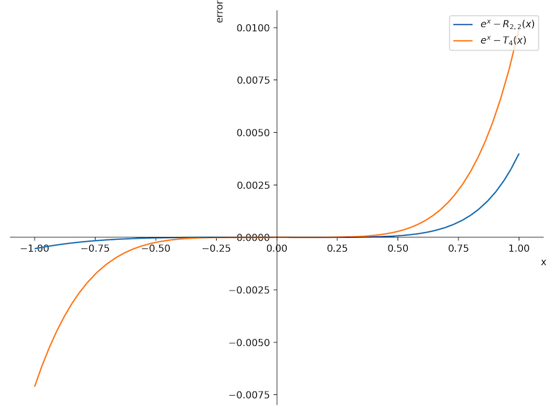
解. 首先, 将函数 \(f(x)\) 表示成 \(4\)-阶 Taylor 展开:\[ e^x=1 + x + \frac{x^{2}}{2} + \frac{x^{3}}{6} + \frac{x^{4}}{24} + O\left(x^{5}\right).\]假设 \(P_2(x)=p_0+p_1x+p_2x^2\) 和 \(Q_2(x)= 1+q_1x+q_2x^2\), 利用定义 (2) 可得\[ \begin{align*} Q_2(x)e^x-P_2(x) &= 1-p_0 + \left( 1+q_1-p_1 \right)x \\ &+ \left( \frac{1}{2}+q_1+q_2-p_2 \right)x^2\\ &+ \left( \frac{1}{6}+\frac{q_1}{2}+q_2 \right) x^3\\ &+ \left( \frac{1}{24}+\frac{q_1}{6}+\frac{q_2}{2} \right) x^4\\ &+ O\left( x^5 \right) \\ \end{align*}\]求解线性系统 (5 个未知数)\[ \begin{align*} 1-p_0&=0,\\ 1+q_1-p_1 &=0,\\ \frac{1}{2}+q_1+q_2-p_2 &=0,\\ \frac{1}{6}+\frac{q_1}{2}+q_2 &= 0,\\ \frac{1}{24}+\frac{q_1}{6}+\frac{q_2}{2} &= 0. \end{align*}\]可得系数 \(p_k, q_k\). 从而 Padé 逼近为\[ R_{2,2}(x) = \frac{12+6x+x^2}{12-6x+x^2}.\]下图中, 画出的是 Padé 逼近 \(R_{2,2}\) 和 Taylor 逼近多项式分别与指数函数的误差, 从中可以看出 Padé 逼近的误差更小. \(\heartsuit\)

例 2 (平方根函数). 求函数 \(f(x)=\sqrt{1+x}\) 的 Padé 逼近 \(R_{2,2}(x)\).

解. 将函数 \(f(x)\) 表示成 \(6\)-阶 Taylor 展开:\[ \sqrt{1+x}=1 + \frac{x}{2} – \frac{x^{2}}{8} + \frac{x^{3}}{16} – \frac{5 x^{4}}{128} + \frac{7 x^{5}}{256} – \frac{21 x^{6}}{1024} + O\left(x^{7}\right).\]假设 \(P_2(x)=p_0+p_1x+p_2x^2\) 和 \(Q_2(x)= 1+q_1x+q_2x^2\), 利用定义 (2) 可得\[ \begin{align*} Q_2(x)f(x)-P_2(x) &= 1-p_0 + \left( \frac{1}{2}+q_1-p_1 \right)x \\ &+ \left( -\frac{1}{8}+\frac{q_1}{2}+q_2 – p_2 \right) x^2\\ &+ \left( \frac{1}{16}-\frac{q_1}{8}+\frac{q_2}{2} \right) x^3\\ &+ \left( -\frac{5}{128}+\frac{q_1}{16}-\frac{q_2}{8} \right) x^4 \\ &+ O\left( x^5 \right) \\ \end{align*}\]求解线性系统 (5 个未知数) 可得\[ R_{2,2}(x) = \frac{16+20x+5x^2}{16+12x+x^2}.\]事实上, 我们可以利用 python (scipy.interpolate.pade) 来计算相应的 Padé 逼近多项式.

from scipy.interpolate import pade
fn = [1.0, .5, -1.0/8.0, 1.0/16.0, -5.0/128, 7/256, -21/1024]
p, q = pade(fn, 3)
# (poly1d([0.109375, 0.875   , 1.75    , 1.      ]),
#  poly1d([0.015625, 0.375   , 1.25    , 1.      ]))

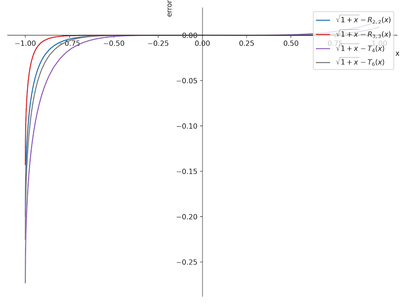
更高阶的 Padé 逼近为 \(R_{3,3}(x) = \frac{0.109375 x^{3} + 0.875 x^{2} + 1.75 x + 1}{0.015625 x^{3} + 0.375 x^{2} + 1.25 x + 1}\). 下图中, 画出的是 Padé 逼近 \(R_{2,2}(x),R_{3,3}(x)\) 和 Taylor 逼近多项式分别与平方根函数的误差, 从中可以看出 Padé 逼近的误差相对更小.

连分式 (Continued fractions)

我们通过一个例子简单了解连分式. 自然对数的基 \(e\) 的连分式 [3] 为\[ e = 2+ \frac{1}{1+ \frac{1}{2+ \frac{1}{1+ \frac{1}{1+ \frac{1}{4 + \frac{1}{1+ \frac{1}{1 + \cdots} } } } } } }, \tag{3}\]通常写成如下简便的形式\[ e = 2+\frac{1}{1+} \frac{1}{2+} \frac{1}{1+} \frac{1}{1+} \frac{1}{4+} \frac{1}{1+} \frac{1}{1+} \frac{1}{6+\cdots}.\]或者写成如下集合的形式\[ e = \left\{ 2,1,2,1,1,4,1,1,6,1,1,8,1,1,10,1,1,12,… \right\},\]

例 3 令 \(f(x):=\sqrt{1+x}\), 那么\[ \sqrt{1+x}=1+\frac{x}{2+ \frac{x}{2+ \frac{x}{2+ \frac{1}{2+ \cdots} } } } \tag{4}\]它的有限逼近为\[ 1+\frac{x}{2}, 1+\frac{x}{2+\frac{x}{2}}, … \tag{5}\]寻找 \(f(x)\) 有理逼近的另外一个方法是通过迭代的形式. 注意到, 函数 \(f(x)\) 不动点方程 \(f(x)=1+\frac{x}{1+f(x)}\) 的解, 我们可以利用如下的不动点算法得到相同的有理逼近:\[ f_{n+1}(x) = 1+\frac{x}{1+f_n(x)},\quad f_0(x) = 1.\]其中, \(f_1(z) = 1+\frac{x}{2}, f_2(z) = 1+\frac{2x}{4+x},\ldots \) 正是连分式 (4) 的截断逼近 (5). 另一方面, 直接计算可得 \(\sqrt{1+x}\) 的 Padé 逼近为\[ R_{1,0}(x)=1+\frac{x}{2},\quad R_{1,1}(x) = 1+\frac{2x}{4+x},\]得到与之前相同的逼近多项式 (5). \(\heartsuit\)

参考

[1] Lorentzen, Lisa. “Padé approximation and continued fractions.” Applied numerical mathematics 60.12 (2010): 1364-1370.
[2] scipy.interpolate.pade.
[3] Kim Milton. Chapter 8. Summation Techniques, Padé Approximants, and Continued Fractions.
[4] J H McCabe. An Observation on the Padé Table for \(\sqrt{1+x}\) and the simple continued fraction expansions for \(\sqrt{2}, \sqrt{3}\) and \(\sqrt{5}\).
[5] Baker, G. A., & Graves-Morris, P. (1996). Padé Approximants (Second Edition).

附录

Python 中的 Padé 逼近

scipy.interpolate.pade(an, m, n=None)
"""
    Return Pade approximation to a polynomial as the ratio of two polynomials.
    
    Parameters
    ----------
    an : (N,) array_like
        Taylor series coefficients.
    m : int
        The order of the returned approximating polynomial `q`.
    n : int, optional
        The order of the returned approximating polynomial `p`. By default,
        the order is ``len(an)-1-m``.

    Returns
    -------
    p, q : Polynomial class
        The Pade approximation of the polynomial defined by `an` is
        ``p(x)/q(x)``.

    Examples
    --------
    >>> from scipy.interpolate import pade
    >>> e_exp = [1.0, 1.0, 1.0/2.0, 1.0/6.0, 1.0/24.0, 1.0/120.0]
    >>> p, q = pade(e_exp, 2)
"""